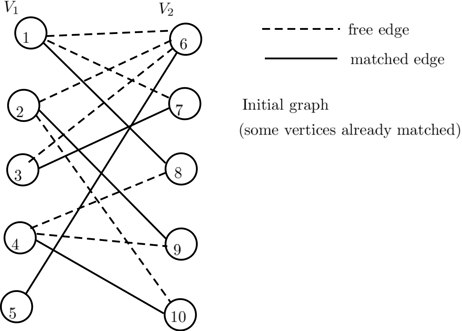
Figure 1.1: Bipartite Graph.
Disclaimer: These notes have not been subjected to the usual scrutiny reserved for formal publications. They may be distributed outside this class only with the permission of the Instructor.
A simple matching occurs when we have set of teachers to assign set of courses to them . Each teacher is qualified to teach certain courses, but not other courses. We assign course to a teacher so that no two teachers are assigned the same course. With a required certain distribution of courses and teachers, it is impossible to assign every teacher a course(s); in that situation we assign as many teachers as possible, and stop when further assignment is not possible.
The figure 1.1 shows this situation, where the vertices are divided into two sets V 1 and V 2, such that vertices in set V 1 represent teachers and those in set V 2 represent courses. When a teacher v ∈ V 1 is qualified to teach a course w ∈ V 2, it is represented by an edge (v,w). Such a graph having vertices in two groups is called bipartite graph. Note that every (v,w) cannot be connected, but only those teachers (v) who are qualified to teach the course (w). All that can be connected in this graph are the free edges (shown as dotted ) plus matched edges (shown as solid lines).
Definition 1.1 Given a graph G = (V,E), a matching M is a subset of the edges such that no two edges in M share a common vertex. In other words, the problem is that of finding a set of independent edges that have no incident vertices in common. The cardinality of M is size of matching.
A task of selecting a maximum subset of such edges is called maximal matching problem. The dark lines in figure 1.1 is one maximal matching in this graph. A complete matching is a matching in which every vertex is an end point of some edge in the matching. Clearly, every complete matching is a maximal matching. Note that the matching shown in figure 1.1 is maximal matching also.
Matching is categorized in two classes: 1) exact matching, which requires a strict correspondence among the two objects being matched or at least any of their sub-parts, 2) Inexact matching, where matching can occur only if two graphs being compared are structurally different to some extent.
A straight forward method to find matchings is to systematically generate all the matchings, and then to pick the one having largest number of edges. But, this has running time as exponential function of number of edges.
The Hall’s Marriage theorem or simply Hall’s theorem, deals with graph theoretic problem using bipartite graph. The following theorem gives necessary and sufficient conditions for existence of a perfect matching in a bipartite graph.
Theorem 1.2 Hall’s theorem: Let G is a bipartite graph, with bipartite sets X and Y , and G = (X,Y,E). For a set W of vertices in X, let Na(W) denote the neighborhood of W in G, i.e., set of all vertices in Y adjacent to some element of W. The marriage theorem in this formulation states that there is a matching that entirely covers X if and only if for every subset W of X:
| (1.1) |
In other words, every subset W of X has sufficiently many adjacent vertices in Y .
Given a finite bipartite graph G = (X,Y,E), with bipartite sets X and Y of equal size, the marriage theorem provides necessary and sufficient conditions for the existence of a perfect matching in the graph.
The above theorem captures exactly the conditions under which a given bipartite graph has a perfect matching, it does not lead to an algorithm for finding maximum matching directly.
For an algorithm for maximal matching, the approach used is called augmenting paths. Let M be the matching. A vertex v is matched if it is an end point of an edge in M.
Definition 1.3 Augmenting Path: A path connecting two unmatched vertices in which two alternate edges are in M is called augmenting path relative to M. The augmenting path must be of odd length, and must begin and end with edges not in M.
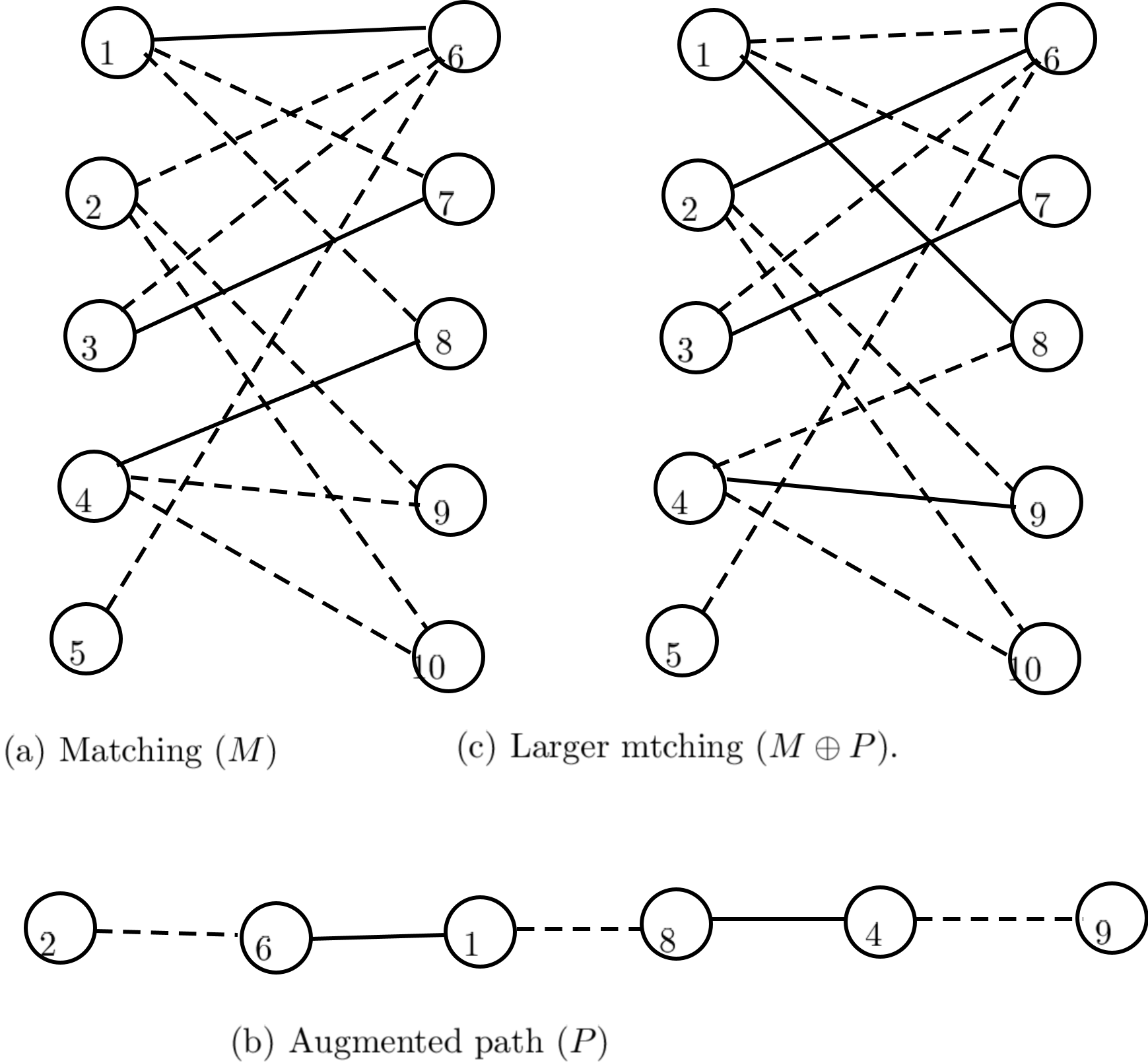
Also, given an augmenting path P, we can always find a bigger matching by removing from M those edges that are in P, and then adding to M the edges of P that were not initially in M. This new matching is M ⊕P, where ⊕ is “exclusive OR” on sets. That is, the new matchings consists of those edges which are in P or M, but not in both.
Lemma 1.4 Let P be the edges on an augmenting path p = [v1,…,vk] with respect to a matching M. Then M′ = M ⊕ P is a matching of cardinality |M| + 1.
Proof. Since P is augmenting path, both v1 and vk are free vertices in M. The number of free edges in P is one more than the number of matched edges. The symmetric difference operator replaces the matched edges of M in P by free edges in P. Hence the size of the resulting matching, |M|′, is one more than |M|. □
Theorem 1.5 A matching in a graph G is maximum matching if and only if there is no augmenting path in G with respect to M.
Proof. The Proof is left as an exercise.
Example 1.6 Figure 1.2(a) shows a graph and a matching M consisting of continuous edges (1,6),(3,7),(4,8). The path 2 → 6 → 1 → 8 → 4 → 9 in figure 1.2(b) shows the augmenting path P. The larger matchings (1,8),(2,6),(3,7),(4,9) in figure 1.2(c) is obtained by removing from M those edges that are in the augmenting path P, and then adding to M the other edges in the path.
The important observation is that M is maximal if and only if there is there is no augmenting path relative to M.
Suppose M and N are matchings with |M| < |N|. Here |M| is number of edges in M. To see that M ⊕N contains an augmenting ptah relative to M, consider the graph G′ = (V,M ⊕N). Since M and N are both matchings, each vertex of V is an end point of at most one edge from M and an end point of one edge from N. Thus each connected component of G′ forms a simple path (possibly cycle) with edges alternating between M and N. Each path that is not a cycle, is either an augmenting path relative to M or augmenting path relative to N depending on whether it has more edges from N or from M. Each cycle has equal number of edges from M and N. Since, |M| < |N|, the exclusive-OR M ⊕ N has more edges from N than M, and hence has at least one augmenting path relative to M.
Following is the algorithm for maximal matchings of M for G = (V,E).
Start with M = ϕ
Find an augmenting path P relative to M and replace M by M ⊕ P.
repeat step 2., until no further augmenting path exists, at this point M is a maximal matching.
It remains only to show how to find an augmenting path relative to matching M. We will do it for simpler case where G is a bipartite graph with vertices partitioned into V 1 and V 2. We build an augmenting path graph for G for levels i = 0,1,2,… using a process similar to BFS (breadth first search). Level 0 consists of all unmatched vertices from V 1. At odd level i, we add new vertices that are adjacent to a vertex at level i - 1, by non-matching edge, and we also add that edge. At even level i, we add new vertices that are adjacent to a vertex at level i - 1 because of an edge in the matching M, together with that edge.
We continue building the augmenting path graph level-by-level until an unmatched vertex is added at an odd level, or until no more vertices can be added. If there is an augmenting path relative to M, an unmatched vertex v will be eventually added at odd level. The path from v to any vertex at level 0 is an augmenting path relative to M.
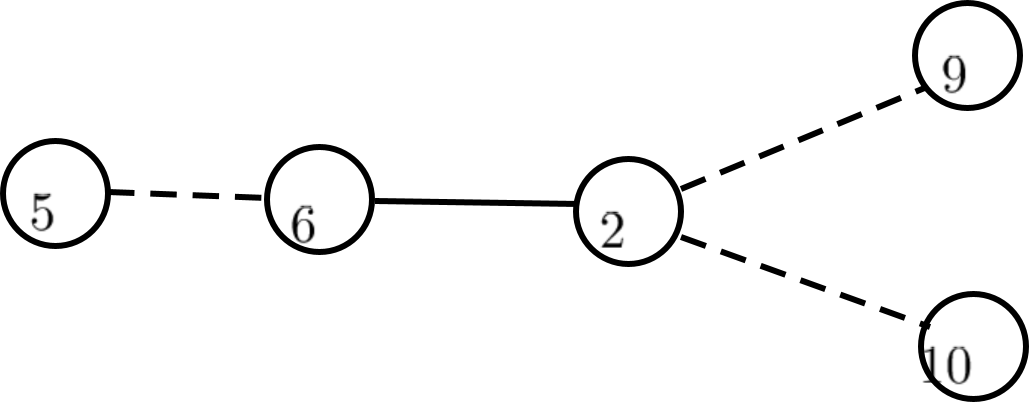
Example 1.7 Figure 1.3 shows the augmenting path graph for the graph of figure 1.2 (a) relative to matching in figure 1.2(c), where vertex 5 has been chosen as unmatched vertex at level 0. At level 1 we add the non-matching edge (5, 6). At level 2 we add the matching edge (6, 2). At level 3 we add either of the non-matching edges (2, 9) or (2, 10). Since both vertices 9 and 10 are currently unmatched, we can terminate the construction of the augmenting path after addition of either of these vertices. Both 9, 2, 6, 5 and 10, 2, 6, 5 are augmenting paths relative to the matching in figure 1.2(c).
Suppose graph G has n vertices and e edges. Constructing the augmenting path graph for a given matching takes O(e) time if the graph was represented as adjacency list representation of edges. To find maximal matching, we construct at most n∕2 augmenting paths, since each enlarges the current matching by at least one edge, and V 1 is V∕2 on the average. Therefore, a maximal matching may be found in O(ne) time for a bipartite graph.
Matchings are the basis of many optimization problems. Problems of assigning workers to jobs can be naturally modeled as bipartite matching problem. Other applications can be assigning a collection of jobs with precedence constraints to two or more processors, such as total execution time is minimized. Other applications are in chemistry, in determining structure of chemical bonds, matching moving objects based on sequence of photographs, and localization of objects in space after obtaining information from multiple sensors.
More applications are as follows:
Finding correspondence between elements of data schemes or data instances.
For example, on merging of two corporations, we want to consolidate their related databases deployed by different departments. For this, a matching of related schemes are required.
Such matchings are also required in other types of schemes, like in UML class taxonomies, ER diagrams, and ontologies.
Matching problems often differ a lot, hence the approach which perform matchings also differ. For example, in matching of relational databases a SQL query could determines which columns are closely related, where as in other matchings hierarchical relationship may be exploited.
In many applications, the crucial operation is the comparison between two objects, or between an object and another to which an object could be related. When structured information is represented by graph, this operation is performed using some form of graph matching. Graph matching is the process finding correspondence between nodes and edges of two graphs that satisfy some constraints ensuring that some substructures in one graph are mapped to similar substructures in another graph.
Write an algorithm to find all the connected components of a graph.
Write an algorithm to determine whether a graph of n vertices has a cycle.
Write an algorithm to find all the simple cycles of a graph. How many such cycles can be there? What is time complexity of this algorithm?
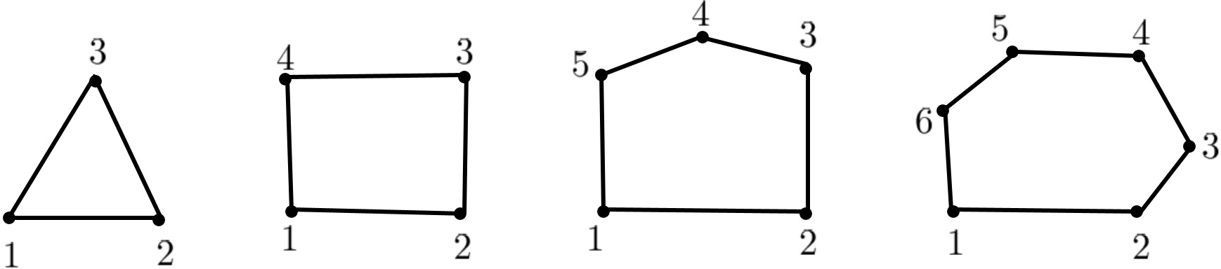
Which of the following graphs are bipartite (figure 1.4)?
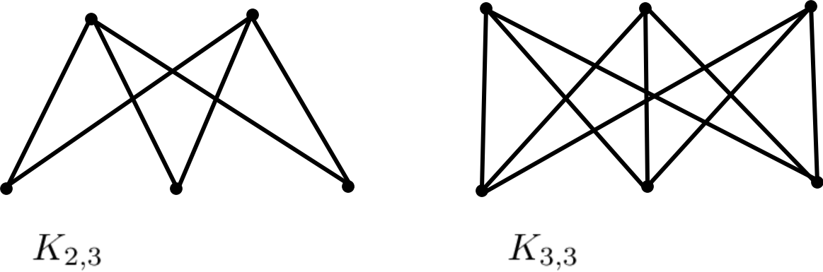
Following are Km,n graphs (figure 1.5)? What is formula for total number of edges in a Km,n graph?
What is maximum number of edges in the maximum matchings of a bipartite graph with n vertices?
Define the terms: maximal matching, maximum matching, perfect matching.
Rewrite the maximal algorithm in your own words.
Determine the complexity of the maximal matching algorithm discussed in the class, and given in this note.
Re-write the algorithm so that it works for minimum matching, instead of maximum matchings.