Ford-Fulkerson method

This section presents a method for solving maximum-flow problem. The method depends on the three important ideas relevant to flow algorithms and problems: residual networks, augmenting paths, and cuts.

The Ford-Fulkerson method iteratively increases the value of the flow. We start with $f(u, v) = 0$ for all $u, v \in V$, giving an initial value of 0. At each iteration, we increase the flow value in $G$ by finding an “augmenting path” in an associated “residual network” $G_R$. Once we know the edges of an augmenting path in $G_R$, we can easily identify specific edges in $G$ for which we can change the flow so that we increase the value of the flow. Although each iteration of the F-F (Ford-Fulkerson) method increases the value of the flow, we shall see that the flow on any particular edge of $G$ may increase or decrease; decreasing the flow on some edges may be necessary in order to enable an algorithm to send more flow from the source to sink in other edge. We repeatedly augment the flow until the residual network has no more augmenting path. The max-flow min-cut theroem will show that upon termination, this process yields a maximum flow (see algorithms ).

We introduce following new concepts, in order to understand the above algorithm.

Residual networks. Given a flow $f$, the residual network $G_R$ consists of edges with capacities that represent how we can change the flow on edge of $G$. An edge of the flow network can admit an amount of additional flow equal to the edge's capacity minus the flow on the edge. If that value is positive ($>0$), we place that edge into $G_R$ with a “residual capacity” $c^\prime(u, v) = c(u,v) - f(u, v)$. The only edges of $G$ that are in $G_R$ are those that can admit more flow; those edges $(u, v)$ whose flow equals their capacity have $c^\prime(u, v) = 0$, and they are not in $G_R$. Note that, in this way, all paths constructed may not be connected.

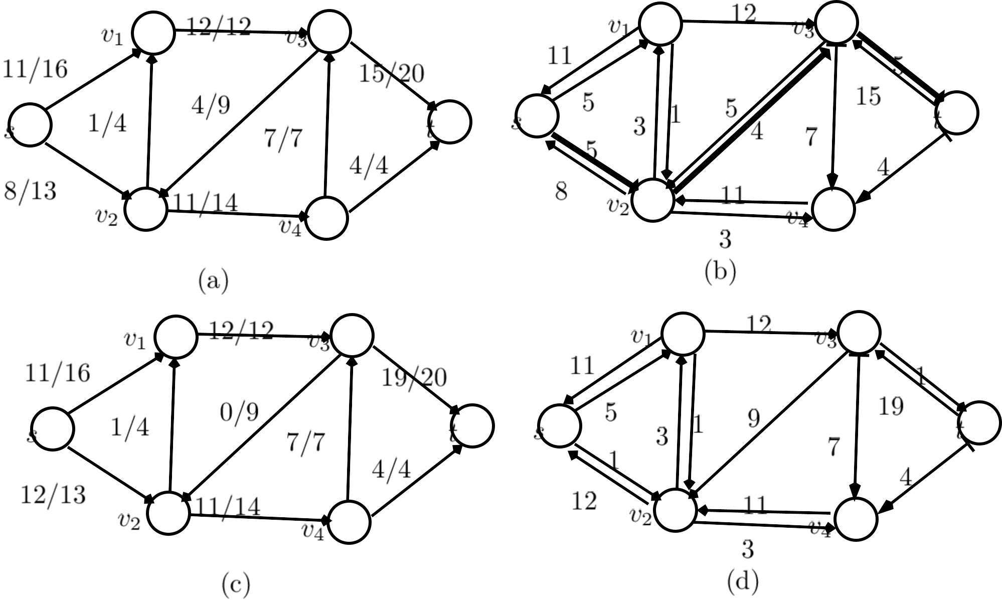
Consider the Figure (a), as a graph $G$ with flows on each edge $(u, v)$ is marked as $a/b$, where $a$ is flow $f(u, v)$ and $b$ is capacity of edge $(u, v)$ expressed as $c(u, v)$. We would now construct a resudual network $G_R$ from $G$.

The residual network $G_R$, may also contain edges that are not in $G$, however. Such edges will be only $(v, u)$ if $(u, v)$ already exists in $G$. As an algorithm manipulates the flow, with the goal of increasing the total flow, it might need to decrease the flow on a particular edge. That is, you can reduce that flow, to the maximum extent which is equal to the original $f(u, v)$, and not more¹. In order to represent a possible decrease of a positive flow $f(u, v)$ on an edge in $G$, we place an edge $(v, u)$ into $G_R$ with residual capacity $c^\prime(u, v) = -f(u, v)$, that is, an edge that can admit flow in the opposite direction to $(u, v)$, at most canceling out the flow on $(u, v)$. These reverse edges in the residual network allow an algorithm to send back flow it has already sent along an edge. Sending flow back along an edge is equivalent to decreasing the flow on the edge, which is a necessary operation in many algorithms. Having completed this operation, the new flow graph is shown in Figure (b). This has been done for all the edges, except those which were running at maximum capacity.

More formally, suppose that we have a flow network $G = (V, E)$ with source $s$ and sink $t$. Let $f$ be a flow in $G$, and consider a pair of vertices $u, v \in V$, we define the residual capacity $c^\prime(u, v)$ by

$$c^\prime(u, v) = \left\{ \begin{array}{ll} c(u, v)-f(u, v), & \te... ...\\ f(v, u), & \text{if} (v, u) \in E,\\ 0, & otherwise.\\ \end{array}\right.$$ (2.6)

Because our assumption that $(u, v) \in E$ implies $(v, u) \notin E$, exactly one case in equation  applies to each ordered pair vertices. As an example, if in this equation, $c(u, v) = 16$ and $f(u, v) = 11$, then we can increase $f(u, v)$ by up to $c^\prime(u, v) = 5$ units before we exceed the capacity constraint on edge $(u, v)$. We also wish to allow an algorithm to return up to 11 units of flow from $v$ to $u$, and hence $c^\prime(v, u) = 11$. This is with $(u, v) = (s, v)$ in figure (b).

Given the flow network $G = (V, E)$ and a flow $f$, the residual network of $G$ induced by $f$ is $G_R = (V, E_R)$, where,

$$E_R = \{(u, v) \in V \times V : c^\prime(u, v) > 0\}.$$ (2.7)

This is as promised above, each edge of the residual network, or residual edge, can admit a flow that is greater than 0.

Figure (a), (b), (c), respectively show the, flow network $G$, residual network $G_R$.

Figure: (a)Flow network $G$ with flow $f$, (b) Residual network $G_R$ with augmenting path $p$ (shaded), its residual capacity is $c^\prime(p) = c^\prime(v_2, v_3) = 4$, edges with residual capacity equal to 0, such as $(v_1, v_3)$, are not shown, (c) The flow in $G$ that results from augmenting along path $p$ by its residual capacity $4$. Edges carrying no flow, such as $(v_3, v_2)$, are labeled by $c(v_3, v_2)$, (d) The residual network induced by the flow in (c).

We increase the flow on $(u, v)$ by $f^\prime(u, v)$ but decrease it by $f^\prime(v, u)$ because pushing flow on the reverse edge in the residual network signifies decreasing the flow in the original network as cancellation. For example, in a data flow network, if we send 5 packets from $u$ to $v$, and send send 2 from $v$ to $u$, we could equivalently just send 3 packets from $u$ to $v$ and none from $v$ to $u$.

In figure (b), we can add the flow in forward direction by difference amount, e.g., on edge $(s, v_2)$ we can add 5 units, and at any time we can undo the forward flow by 8 units.

After augmenting graph in figure (a) with the augmenting path $s\rightarrow v_2 \rightarrow v_3 \rightarrow t$, having augmented flow of $4$, it cancels existing flow in edge $(v_3, v_2)$, hence flow in edge $(v_3, v_2)$ is zero.